
Documentation
Getting Started
GRNsight is a web application for visualizing models of small-scale gene regulatory networks (GRNs) or protein-protein interaction networks (PPIs). GRNsight was originally created to work with the input and output spreadsheets used by GRNmap, a MATLAB program that estimates the parameters and performs forward simulations of a differential equations model of a GRN. However, GRNsight can be used to visualize any small-scale GRN or PPI that is specified by the appropriate Excel workbook format. GRNsight is best-suited for visualizing networks of fewer than 35 nodes (genes/proteins) and 70 edges (regulatory relationships/binding interactions), but can display networks of up to 75 nodes and 150 edges. Although originally designed for gene regulatory networks, we believe that GRNsight has general applicability for displaying any small, unweighted or weighted network with directed or undirected edges for systems biology or other application domains. The following sections describe how to use GRNsight.
GRNsight has been tested with and confirmed to be working in Chrome version 146.0.7680.154 or higher and Firefox version 148.0.2 or higher on Windows 11 and macOS 26 Tahoe operating systems. It may not work with other browsers, versions, or operating systems.
-
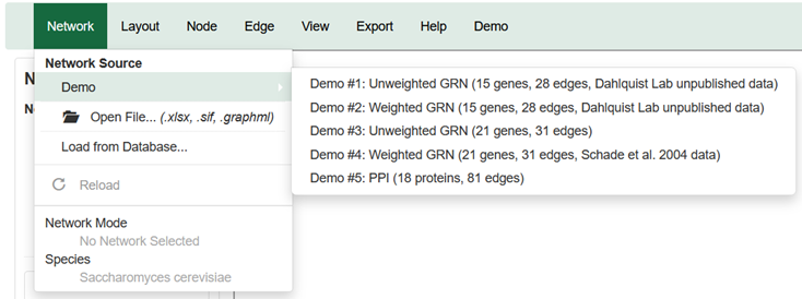
The Network menu or sidebar panel are used to load a network into GRNsight. There are three ways to load a network into GRNsight:
-
You can load a network from one of our available Demo files, as explained in Section 1a.
-
You can create and load a GRNsight-compatible input workbook (*.xlsx), SIF file (*.sif), or GraphML (*.graphml) file, as explained in Section 1b.
-
You can create and load a network for Saccharomyces cerevisiae from genes/proteins stored in our Network Database, as detailed in Section 1c.
-
You can load a network from one of our available Demo files, as explained in Section 1a.
- Once a network is loaded, the Network Mode shown in the Network menu or sidebar panel will change from No Network Selected to either Gene Regulatory Network or Protein-Protein Interaction, depending on the type of network loaded.
- The Species displayed in the Network menu or sidebar panel will show Saccharomyces cerevisiae to remind the user that GRNsight defaults to displaying networks from budding yeast. However, a user that uploads their own network can display data from any species (see Section 1b).
If you do not have your own input spreadsheet, you can load and view demonstration gene regulatory and protein-protein physical interaction networks.
-
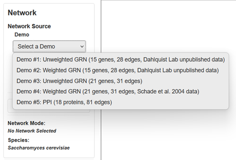
You can access the demo selections from the Network menu across the top of the window and from the Network panel on the side bar.
-
You can select from among five demo networks:
- Demo #1: Unweighted GRN (15 genes, 28 edges, Dahlquist Lab unpublished data) is a gene regulatory network that displays black edges with pointy arrowheads. Nodes are colored with timecourse gene expression data for budding yeast subjected to cold shock at 13°C for 15, 30, and 60 minutes (GSE83656).
- Demo #2: Weighted GRN (15 genes, 28 edges, Dahlquist Lab unpublished data) is a gene regulatory network that displays colored edges of varied thickness with pointy or blunt arrowheads. Nodes are colored with timecourse gene expression data for budding yeast subjected to cold shock at 13°C for 15, 30, and 60 minutes (GSE83656). Edge weights were modeled with the GRNmap software.
- Demo #3: Unweighted GRN (21 genes, 31 edges) is a gene regulatory network that displays black edges with pointy arrowheads. Nodes are colored with timecourse gene expression data for budding yeast subjected to cold shock at 10°C for 0, 10, 30, and 120 minutes (https://doi.org/10.1091/mbc.e04-03-0167)
- Demo #4: Weighted GRN (21 genes, 31 edges, Schade et al. 2004 data) is a gene regulatory network that displays colored edges of varied thickness with pointy or blunt arrowheads. Nodes are colored with timecourse gene expression data for budding yeast subjected to cold shock at 10°C for 0, 10, 30, and 120 minutes (https://doi.org/10.1091/mbc.e04-03-0167). Edge weights were modeled with the GRNmap software, as reported in Dahlquist et al. (2015).
- Demo #5: PPI (18 proteins, 81 edges) is a protein-protein physical interaction network that displays black, undirected edges. It represents proteins that interact with the budding yeast protein Aim32p curated by the Saccharomyces Genome Database.
- See Section 2 for more details on how GRNsight displays the graph.
-
To reload the same demo, select the top menu option Network > Network Source > Reload or click the Reload button in the Network side bar panel. Note that the Reload menu item will be disabled until a file has been loaded.
- If you have a Microsoft Excel workbook file (*.xlsx) that was used as an input or generated as an output by the MATLAB program GRNmap, you do not need to perform any further modifications to use the workbook with GRNsight. You can move on to Section 1b-ii to learn how to open your file.
If you want to create manually a new file to use with GRNsight, format the file in the following manner:
-
GRNsight accepts Microsoft Excel workbook (*.xlsx) files as its native format.
- Note that Excel 97-2003 workbook (*.xls) files are not able to be read by GRNsight.
- If you have a SIF (*.sif) or GraphML (*.graphml) file, please see Section 1b-i.c or Section 1b-i.d, respectively, to verify that your files are formatted correctly for import into GRNsight.
-
GRNsight reads gene regulatory network or protein-protein interaction network information that is in the form of an adjacency matrix to generate the nodes and edges of the graph.
- There must be one worksheet in your Excel workbook entitled “network” or “network_optimized_weights”. Generally, the “network” worksheet describes an unweighted network (either GRN or PPI) and the “network_optimized_weights” worksheet describes a weighted network (GRN-only). If the workbook contains worksheets with both names, the display of the “network_optimized_weights” data will take precedence.
- For a GRN, in the “network” and “network_optimized_weights” worksheets, the upper-left cell (A1) should contain the text “cols regulators/rows targets”. This text is there as a reminder of the direction of the regulatory relationships specified by the adjacency matrix. For a PPI, in the "network" sheet, cell A1 should contain the text "cols protein1/rows protein2"
- For a GRN, the rest of the first row should contain the names of the transcription factors that are controlling the other genes in the network, one transcription factor name per column. Transcription factor names must be unique for each column and must be 12 characters or fewer. For PPI networks, protein names of 12 characters or fewer are used instead.
- For a GRN, the rest of the first column should contain the names of the target genes that are being controlled by the transcription factors heading each of the columns in the matrix, one target gene name per row. Transcription factor names must be unique for each row and must be 12 characters or fewer. For PPI networks, protein names of 12 characters or fewer are used instead.
- With respect to GRNs, GRNsight is primarily designed to depict gene regulatory networks that contain just transcription factors and that can be represented by a symmetric adjacency matrix. However, starting with version 1.8, GRNsight allows the user to upload spreadsheets with asymmetric adjacency matrices. I.e., the number, identity, and order of genes across the top and side of the adjacency matrix do not have to match. A gene name at the top of the matrix will be considered the same as a gene name on the side if it contains the same text string, regardless of capitalization. For example, “ACE2”, “Ace2”, and “ace2” would all be considered the same gene, but “ACE_2” or “ACE-2” would not be considered the same as “ACE2”. Gene names may not contain any special characters other than "-" and "_". GRNsight is case-preserving in that it will keep the capitalization that the user originally entered into the spreadsheet. The gene name capitalization occurring across the top takes precedence over the gene name capitalization occurring on the side of the adjacency matrix for display of the gene names on the nodes of the graph. The nodes that display on the graph are automatically sized to accommodate the size of the label. Labels are restricted to 12 characters; use shorter gene symbols for nodes so that the node boxes do not get too large. For PPIs, these same rules apply.
-
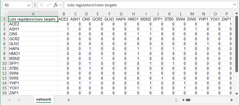
For unweighted GRN networks, in the “network” worksheet, each cell in the matrix should then contain a zero (0) if there is no regulatory relationship between those two transcription factors, or a one (1) if there is a regulatory relationship between them. In the screenshot below, the “1” in cell B3 means that ACE2 regulates ASH1. The “1” in cell H8 means that HMO1 regulates itself. When this file is loaded into GRNsight, it will generate a graph with 15 nodes, one for each transcription factor, and 28 edges, for each of the cells that contain a “1” in this adjacency matrix. The edges will be black with regular (pointy) arrowheads. The demonstration file "Demo #1: Unweighted GRN (15 genes, 28 edges, Dahlquist Lab unpublished data)" contains the adjacency matrix shown below. Follow the link to download the file.
-
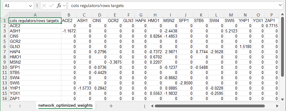
For a GRN, when GRNsight encounters a worksheet entitled “network” with all 1’s and 0’s specifying an adjacency matrix, it will automatically color the edges black and put regular (pointy) arrowheads on the edges. However, GRNsight can also be used to display weighted edges with varying thicknesses and colors based on the magnitude and sign of the weights, respectively. To generate this type of adjacency matrix by hand, create a worksheet called “network_optimized_weights”. Instead of using 1’s to indicate connections in the network, use values that are real numbers > 0 to indicate an activation relationship or < 0 to indicate a repression relationship. The screenshot below gives an example of this type of adjacency matrix. The demonstration file Demo #2: Weighted GRN (15 genes, 28 edges, Dahlquist Lab unpublished data) contains the adjacency matrix shown below. Follow the link to download the file. For the weighted edges to display with different colors and thicknesses, make sure that you have selected the menu item Edge > Enable Edge Coloring Based on Weight Values from the top or side-bar menu. For more information on how GRNsight displays weighted edges on the graph, see Section 2 below.
- Note that GRNsight is designed to visualize “small-scale” gene regulatory or protein-protein interaction networks, not the entire gene network for an organism. Currently, it is recommended that you upload networks with no more than 35 unique genes/proteins or 70 edges. If you upload a network with 50 nodes or 100 edges or more, you will receive a warning and the network graph will still display. If you attempt to upload a network of 75 or more nodes or 100 or more edges, the graph will not display.
- Follow these instructions to download and format a regulation matrix from the YEASTRACT database for use with GRNsight.
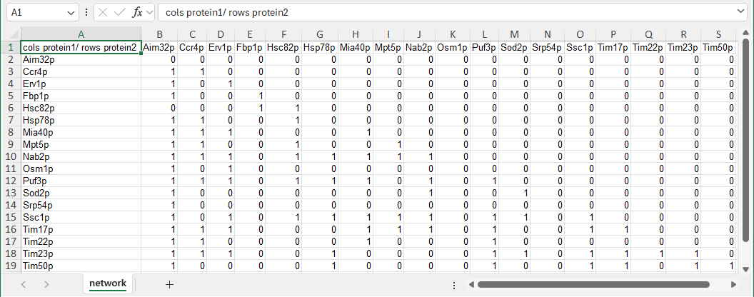
- Starting in v7.1.2 GRNsight can display protein-protein interaction networks. Format the "network" sheet as described above for GRNs, except column A1 should have the text "cols protein1/rows protein2". Since PPIs have undirected edges, a “1” indicates a binding interaction between two proteins or a protein and itself. The demonstration file Demo #5 PPI (18 proteins, 81 edges) is shown below. Follow the link to download the file. Note that currently, GRNsight does not support displaying weighted edges for PPIs.
-
Starting in v3.0.0, GRNsight reads in time series expression data from worksheets in the Excel workbook, and displays these data as heat maps on individual nodes with one vertical stripe per timepoint.
-
Demo #1 Unweighted GRN (15 genes, 28 edges, Dahlquist Lab unpublished data) and Demo #2 Weighted GRN (15 genes, 28 edges, Dahlquist Lab unpublished data) have examples of how these worksheets should be formatted (shown below). Follow the links to download the files.
- In brief, Excel worksheets with names ending with "_log2_expression" are processed as time series expression data. Multiple expression worksheets with unique names can be included in the workbook. For example "wt_log2_expression" or "dcin5_log2_expression".
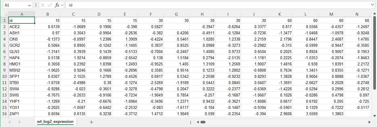
- The upper-left cell (A1) should contain the text “id”.
-
Demo #1 Unweighted GRN (15 genes, 28 edges, Dahlquist Lab unpublished data) and Demo #2 Weighted GRN (15 genes, 28 edges, Dahlquist Lab unpublished data) have examples of how these worksheets should be formatted (shown below). Follow the links to download the files.
- The rest of the first column should contain the names of the genes, one gene name per row. Gene names must be unique for each row and must be 12 characters or fewer. These names must be identical to the names contained on the "network" and/or "network_optimized_weights" sheets and in the same order.
- The rest of the first row should contain numerical time points in ascending order; do not include units. Replicates of the same time point are indicated by repeating the same numerical time point header for each replicate. When displaying the heat map on the node, you will have the option of displaying one stripe for each time point and replicate or averaging values for the same replicate to create one stripe per timepoint.
- Subsequent rows should contain the log2 expression value of that particular gene at the given time point (and replicate, if applicable). Blank cells are allowed, indicating the lack of a data point for a particular transcription factor at a given time. For example, in the image of the "wt_log2_expression sheet", cells G2 and N16 are blank because data are missing for those replicates and timepoints.
- Please see Section 2e for more information on how to interpret and manipulate the node coloring visualization.
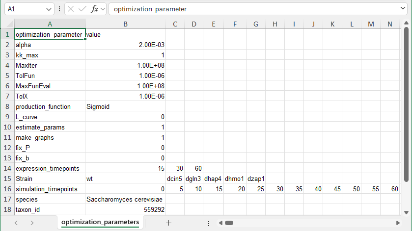
- In brief, the first row should contain the headers “optimization_parameter” in cell A1 and “value” in cell B1.
- In the first column, the following optimization parameters appear in this order: “alpha”, “kk_max”, “MaxIter”, “TolFun”, “MaxFunEval”, “TolX”, “production_function”, “L_curve”, “estimate_params”, “make_graphs”, “fix_P”, “fix_b”, “expression_timepoints”, “Strain”, “simulation_timepoints”, “species”, “taxon_id”, and “workbookType”.
- The value in column B for the following parameters is a real number: “alpha”, “kk_max”, “MaxIter”, “TolFun”, “MaxFunEval”, and “TolX”.
- The value in column B for the following parameters is an integer, either “0” or “1”: “L_curve”, “estimate_params”, “make_graphs”, “fix_P”, and “fix_b”.
- The value in column B for the following paramters is a string: “production_function” and “species”.
- The following optimization parameters can be a list of numbers: “expression_timepoints” and “simulation_timepoints”, one number per column to the right starting in column B. The “expression_timepoints” should correspond to the timepoints in the “_log2_expression” sheets.
- The following optimization parameter can be a list of strings, one string per column to the right starting in column B: “Strain”. These correspond to the prefix to the worksheet names containing the timecourse expression data. For example, if your workbook contains sheets named “wt_log2_expression” and “dcin5_log2_expression”, the values would be “wt” and “dcin5”.
- Navigate to Generate Regulation Matrix on the YEASTRACT site.
- Select the appropriate radio buttons/check boxes for the filters.
- Paste a list of transcription factors into the appropriate field.
- Paste a list of targets into the Target ORF/Genes field, or check the box to consider all ORF/Genes.
- Click the Generate button.
- In the results window that appears, click the link to download the Regulation matrix results file as a Semicolon Separated Values (CSV) file (not the Two-column table, Tab Separated Values (TSV) file).
- Once you have downloaded the file, launch Microsoft Excel.
- Select the menu item, File > Open and select the file that you downloaded.
- Select Column A.
- Select the menu item, Data > Text to Columns...
- In the first window of the wizard that appears, select the radio button for "Delimited" and click Next.
- In the second window of the wizard that appears, check the box for "Other" under "Delimiters" and type a semicolon in the field to the right and click Finish.
- Select the menu item, File > Save As... and save the file as an Excel workbook (.xlsx).
- YEASTRACT organizes the adjacency matrix with the transcription factors as rows and the target genes as columns, which is opposite to the format that GRNmap and GRNsight expects. To flip this orientation, first create a new worksheet by clicking on the new worksheet icon at the bottom of the screen. Name this new worksheet "network".
- Select the adjacency matrix from the first worksheet and copy it to the clipboard. Go to the "network" worksheet and click on cell A1. Select the menu item Edit > Paste Special. In the window that appears, check the box "Transpose" and click OK.
- The labels for the genes in the columns and rows needs to match. Thus, delete the "p" from each of the gene names in the columns.
- Paste the following text into cell A1 "cols regulators/rows targets".
- Save your work. This file is now ready for loading into GRNsight. You can choose to delete the original worksheet or keep it in your workbook.
- A SIF file is a tab-delimited text file with the file extension .sif.
- Note that the Cytoscape SIF specification also allows space-delimited files. However, due to the confusion caused when a space character is used in a node label or interaction type, GRNsight only allows tabs as delimiters for .sif files.
- Lines in the SIF file specify a source node, a relationship type (or edge type), and one or more target nodes separated by tab characters.
- For a network defined in SIF format, node names should be unique, as identically named nodes will be treated as identical nodes.
- Node names must be 12 characters or fewer.
- Starting in GRNsight v2, the relationship type for an unweighted GRN is required to be "pd". "pd" was chosen because it commonly means protein -> DNA (e.g. a regulatory transcription factor binding upstream of a target gene) in the systems biology community. A strict requirement for the relationship type was specified to expand upon SIF syntactic error checking capabilities.
- Starting in GRNsight v7, protein-protein interaction networks are supported. The relationship type for an unweighted PPI is required to be "pp", for "protein-protein".
- Duplicate entries are ignored (as would occur if the same source-target pair was listed twice with two different relationship types).
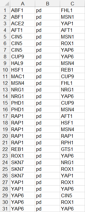
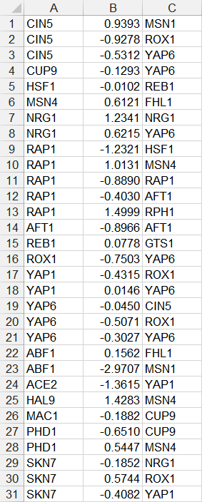
- GRNsight automatically detects whether the SIF file represents an unweighted or weighted GRN or PPI network through the examination of the relationship type. The screenshots and descriptions below are four valid ways that an unweighted GRN can be specified as a SIF file, using the file Demo #3: Unweighted GRN (21 genes, 31 edges)" as an example. (The screenshots display a tab-delimited text file as it would be displayed in Microsoft Excel.) Follow the link to download a sample SIF file.
- In the first example below, each source node in the network is listed in the first column, the relationship type “pd” is listed in the second column, and the target node is listed in the third column. If a node has multiple target nodes, it is listed multiple times, one relationship per line. A node may regulate itself (for example, AFT1). Note that FHL1, GTS1, MSN1, and RPH1 do not have any target nodes, but are still listed as source nodes. While they can be listed, it is not necessary to do so, as is shown in the second example.
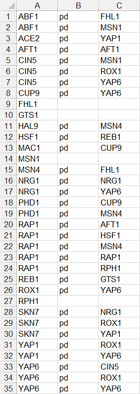
- In the second example below, only source nodes that have target nodes are listed in the first column, the relationship type “pd” is listed in the second column, and the target node is listed in the third column. If a node has multiple target nodes, it is listed multiple times, one relationship per line. (FHL1, GTS1, MSN1, and RPH1 were removed because they did not have any target nodes.)
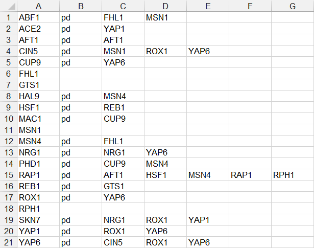
- In the third example below, each source node is only listed once on one line, followed by the relationship type “pd”, followed by a series of target nodes, separated by tab characters. Note that FHL1, GTS1, MSN1, and RPH1 do not have any target nodes, but are still listed as source nodes. While they can be listed, it is not necessary to do so, as is shown in the fourth example.
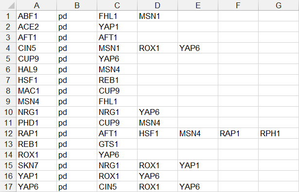
- In the fourth example below, each source node is only listed on one line, followed by the relationship type “pd”, followed by a series of target nodes, separated by tab characters. (FHL1, GTS1, MSN1, and RPH1 were removed because they did not have any target nodes.)
- A Cytoscape SIF file is only intended to convey the network nodes and edge connections; it does not support the storage of other node or edge attributes or display properties. However, with a modification to the relationship type, a SIF file can represent a weighted GRN and be displayed as such in GRNsight upon import (See Section 2a).
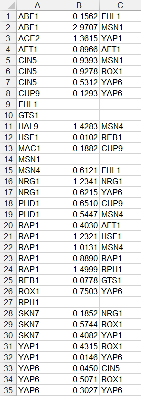
- To encode a weighted network in a SIF file, instead of using a text string like “pd” as the relationship type, substitute the numerical weight value. Use real numbers > 0 to indicate an activation relationship or < 0 to indicate a repression relationship. The screenshots and descriptions below are two valid ways that a weighted network can be specified as a SIF file, using the file Demo #4: Weighted GRN (21 genes, 31 edges, Schade et al. 2004 data)" as an example. (The screenshots display a tab-delimited text file as it would be displayed in Microsoft Excel.) Follow the link to download a sample SIF file.
- In the first example below, each source node in the network is listed in the first column, the numerical value of the weight is listed in the second column, and the target node is listed in the third column. If a node has multiple target nodes, it is listed multiple times, one relationship per line. Note that FHL1, GTS1, MSN1, and RPH1 do not have any target nodes, but are still listed as source nodes. While they can be listed, it is not necessary to do so, as is shown in the second example.
- In the second example below, only source nodes that have target nodes are listed in the first column, the numerical value of the weight is listed in the second column, and the target node is listed in the third column. If a node has multiple target nodes, it is listed multiple times, one relationship per line. (FHL1, GTS1, MSN1, and RPH1 were removed because they did not have any target nodes.)
- For a weighted network, each source-to-target relationship should be on a separate line. While it is possible that two or more source-to-target relationships would have the same exact weight value, it is not recommended to use the shorthand of listing multiple target nodes on the same row.
- GRNsight will automatically detect a SIF file representing a weighted GRN when it finds numerical values as the relationship type. It will change the arrowhead type and the thickness and color of the edges as described in Section 2a.
- However, if it detects a mix of numerical and "pd" string values as the relationship type, it will issue a warning to the user that this was detected, but still display the network as an unweighted GRN.
- If the user has deselected the menu item Edge > Enable Edge Coloring Based on Weight Values, GRNsight will ignore the numerical weight values and display the network as an unweighted graph.
- Note that these “weighted” SIF files are able to be imported in to Cytoscape (tested with v3.4.0), but the weight values will not be properly stored as edge attributes by Cytoscape because it does not use the SIF format in this way.
- The display of PPI networks does not support weighted edges. A PPI SIF file can be specified the same way as in the first three examples, except “pp” is used instead of “pd”
- Note that GRNsight is designed to visualize “small-scale” gene regulatory or protein-protein interaction networks, not the entire network for an organism. Currently, it is recommended that you import networks with no more than 35 unique genes or 70 edges. If you upload a network with 50 nodes or 100 edges or more, you will receive a warning and the network graph will still display. If you attempt to upload a network of 75 or more nodes or 100 or more edges, the graph will not display.
Users who have GRN data in GraphML format can import these files directly into GRNsight. However, if you are creating a new input file for use with GRNsight, we recommend using the native Excel format expected by GRNsight as described in Section 1a. GRNsight does not currently support import of PPI networks in GraphML format.
A primer for the GraphML format can be found at http://graphml.graphdrawing.org/primer/graphml-primer.html, whereas the detailed specification can be found at http://graphml.graphdrawing.org/specification.html. The instructions below borrow heavily from the GraphML primer.
- A GraphML file is an Extensible Markup Language (XML) file with the extension .graphml.
- GraphML has the ability to specify graph features that GRNsight cannot display. In those cases, GRNsight will ignore the features that it does not support.
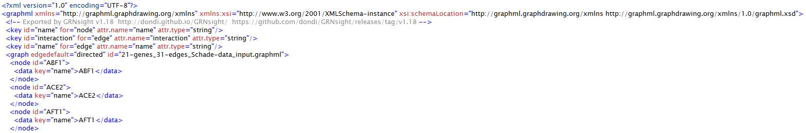
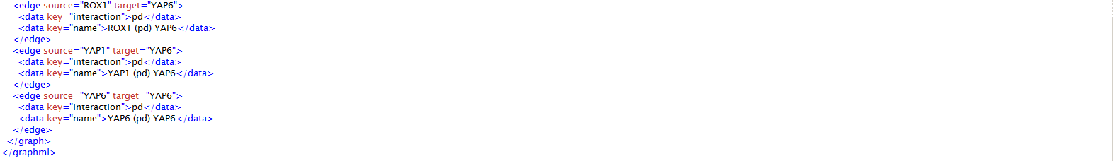
- The minimum requirements for an unweighted GRN GraphML file that GRNsight can read and display is best illustrated by an example. The screenshots below show the top and bottom of the Demo #3 Unweighted GRN (21 genes, 31 edges) GraphML file as exported by GRNsight. (The screenshots were created from a view of this file in the firstobject XML Editor). Click the link to download the file.
...
- “The first line of the document is an XML process instruction which defines that the document adheres to the XML 1.0 standard and that the encoding of the document is UTF-8, the standard encoding for XML documents.”—GraphML Primer
- “The second line contains the root-element element of a GraphML document: the
graphmlelement. The graphml element, like all other GraphML elements, belongs to the namespacehttp://graphml.graphdrawing.org/xmlns. For this reason we define this namespace as the default namespace in the document by adding the XML Attributexmlns="http://graphml.graphdrawing.org/xmlns"to it. The two other XML Attributes are needed to specify the XML Schema for this document. In our example we use the standard schema for GraphML documents located on thegraphdrawing.orgserver. The first attribute,xmlns:xsi="http://www.w3.org/2001/XMLSchema-instance", definesxsias the XML Schema namespace. The second attribute,xsi:schemaLocation="http://graphml.graphdrawing.org/xmlns http://graphml.graphdrawing.org/xmlns/1.0/graphml.xsd", defines the XML Schema location for all elements in the GraphML namespace.”—GraphML Primer - The third line is a comment injected by GRNsight, giving the name of the program that created the document (GRNsight), the version (in this case v1.18), URL of the GRNsight home page, and URL to the GitHub release page for the specified version. This information is provided upon export of a GraphML file by GRNsight to assist with keeping track of the provenance of the data, and is optional for the import of GraphML files into GRNsight.
- The next three lines are key elements. GraphML standardizes only the representation of nodes and edges and their directions; all other characteristics, such as names, weights, and other values, are left for others to specify through a key element, which is not subject to a controlled vocabulary. For an unweighted network, GRNsight-exported GraphML defines the keys:
- name for the node label (The node name is defined for compatibility with Cytoscape, but is optional for GRNsight to read and display the graph.)
- interaction for the relationship type of the edge (The relationship type is defined in the same way as for SIF files described in Section 1c for compatibility with Cytoscape, but is optional for GRNsight to read and display the graph.)
- name for the edge (The edge name is defined for compatibility with Cytoscape, but is optional for GRNsight to read and display the graph.)
- "A graph is, not surprisingly, denoted by a
graphelement. Nested inside agraphelement are the declarations of nodes and edges. A node is declared with anodeelement, and anedgewith an edge element."—GraphML Primer - In the graph element in line 7, the edgedefault attribute is set to “directed”. GRNsight will only display directed graphs, not undirected or mixed graphs.
- The id attribute gives the name of the GraphML file, and is optional for GRNsight to read and display the graph. The id is provided for compatibility with Cytoscape.
- The next three elements in the screenshot are node declarations, giving an id and name for the nodes “ABF1”, “ACE2”, and “AFT1”.
- Note that for GRNsight-exported GraphML, the node id and name are identical and unique to the file. However, other programs may have a node name that is different than the node id. For example, both Cytoscape v3.4.0 and yED v3.16 assign internal node identifiers that the user cannot edit. The user does have the ability edit the node label, and it is for this reason that GRNsight will preferentially display the node label on the graph. However, user editability in Cytoscape and yED leads to a situation where a user can actually assign the same label to two different nodes. In this case, duplicate node labels will be displayed by GRNsight, and the user is directed to go back and edit the source file.
- Cytoscape uses the name key to assign a label to nodes and a shared name key to assign a label to the root network when subnetworks are present.
- yED uses a y:NodeLabel key to assign the label to nodes.
- In order to maximize the ability for GRNsight to read GraphML exported from Cytoscape and yED, the following conditions are followed when displaying a graph: if all three keys are present name gets top priority, followed by shared name, then y:NodeLabel, then id.
- The next three elements shown in the screenshot are edge declarations for the edges ROX1-to-YAP6, YAP1-to-YAP6, and YAP6-to-YAP6.
- The edge element attributes source and target give the node id for the source and target node, respectively.
- The interaction key is the relationship type, similar to what is defined for SIF files. It is given for compatibility with Cytoscape and defaults to “pd” for protein->DNA, but is otherwise ignored by GRNsight for display.
- The edge name key is given for compatibility with Cytoscape, but is otherwise ignored by GRNsight for display.
- As noted above, GraphML has the ability to specify graph features that GRNsight cannot display. In those cases, GRNsight will ignore these features. The original imported file will not be changed, but a GRNsight re-export of the same graph will omit these elements.
- GRNsight cannot display a nested graph. Any links that connect nodes from the main graph to nodes in the subgraph will not display.
- Any other specifications for the display of the graph (layout, colors, etc.) will be ignored by GRNsight.
- We have tested the display of networks exported in GraphML format from Cytoscape v3.4.0 and yED v3.16, but because the flexibility of the GraphML standard enables divergence in implementation, we cannot guarantee that GraphML exported from other programs will be read and displayed correctly by GRNsight. If you encounter problems, please submit an issue to GRNsight @ GitHub (requires free GitHub account).
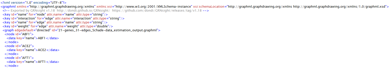
- The minimum requirements for a weighted GRN GraphML file that GRNsight can read is best illustrated by an example. The screenshots below show the top and bottom of the Demo #4 Weighted GRN (21 genes, 31 edges, Schade et al. 2004 data) GraphML file as exported by GRNsight. Click the link to download the file.
...
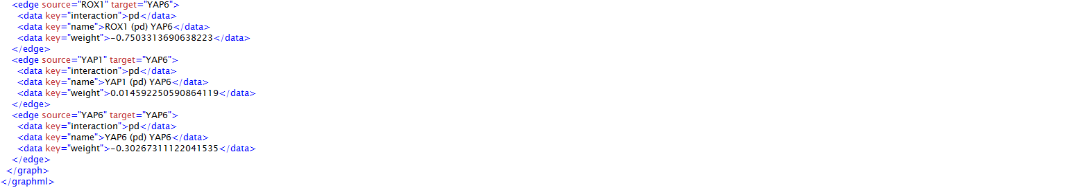
- Note that there are only two major differences between the unweighted and weighted GRN GraphML formats that GRNsight exports:
- A key declaration defining a weight attribute for an edge as the datatype “double”.
- Note that there is a bug in Cytoscape v3.4.0 with the way it exports GraphML files. It currently assigns the weight attribute for a node instead of an edge. To maximize the ability for GRNsight to read and display Cytoscape-exported GraphML, GRNsight does not currently enforce that the weight attribute be declared "for an edge". The bug has been reported to the Cytoscape group.
- The addition of the weight key for each edge. For example, the weight for the edge ROX1-to-YAP6 is -0.7503313690638223.
- GRNsight automatically detects if a GraphML file specifying a weighted GRN graph has been imported.
- For a weighted GRN graph to display, the weight attribute must be present and valid for all edges declared in the graph. If one or more weights are missing, GRNsight will display the graph as unweighted with black edges and pointed arrowheads.
- Note that GRNsight is designed to visualize “small-scale” gene regulatory or protein-protein interaction networks, not the entire network for an organism. Currently, it is recommended that you import networks with no more than 35 unique genes or 70 edges. If you upload a network with 50 nodes or 100 edges or more, you will receive a warning and the network graph will still display. If you attempt to upload a network of 75 or more nodes or 100 or more edges, the graph will not display.
- Once you have your appropriately formatted Excel workbook (*.xlsx), SIF (*.sif), or GraphML (*graphml) file, you can load it into GRNsight.
-
Go to the GRNsight home page. Select the top menu option Network > Network Source > Open File...(.xlsx., .sif, .graphml). A dialog box will open for you to select your file. Clicking the Open button will load your file. Clicking the Cancel button will return you to the GRNsight home page. Alternately, you can use the Open File button in the Network > Network Source side panel.
- The name of the file that is currently loaded will appear in the menu bar. The number of nodes and edges in the graph will display on the right-hand side of the menu bar.
- To load a different file, select the menu option Network > Network Source > Open File...(.xlsx., .sif, .graphml) or click the Open File button in the Network > Network Source side panel. The previously loaded file is not saved, and only the newly selected file will display.
-
To reload the same file, select the top menu option Network > Network Source > Reload or click the Reload button in the Network side bar panel. Note that the Reload menu item will be disabled until a file has been loaded.
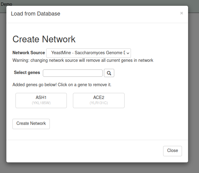
If you do not have your own input network, you can use the Load from Database feature to select genes/proteins from our backend Saccharomyces cerevisiae database derived from the Saccharomyces Genome Database and display them as a gene regulatory or protein-protein physical interaction network.
-
To access the Load from Database feature, select the side bar or top menu item Network > Network Source > Load From Database. A pop up Generate Network window will appear. Select the Network Type, either Gene Regulatory or Protein-Protein Physical Interactions from the drop-down menu. Choose the Network Source from the drop-down menu. GRNsight updates its backend database once a year, obtaining data from the Saccharomyces Genome Database via Yeastmine (2022, 2023, and 2024) or AllianceMine (2025 and onwards). Older versions of the database can be selected to maintain reproducible results from previous work. Select genes (for a GRN) or proteins (for a PPI) by typing either the yeast standard name or systematic name into the Select field and clicking the magnifying glass button or hitting the Enter key on your keyboard. Once found, the genes/proteins will appear listed below the search field. To remove a gene/protein, left-click on it, and it will be removed from the list. Changing the Network Type or Network Source selection will clear the list of selected genes or proteins. Once complete, click on the Generate Network button and the selected gene regulatory or PPI network will be displayed by GRNsight. Clicking the cancel button will close the window without displaying a new network graph.
GRNsight graphs are generated through D3.js, a JavaScript data visualization library. We have modified the default implementation of D3 to include the following features:
- Nodes are rectangular.
- The labels on the nodes are what is found in your “network” or “network_optimized_weights” worksheet, depending on whether you are displaying an unweighted or weighted graph. GRNsight is case-preserving in that it will keep the capitalization that the user originally entered into the spreadsheet. The gene name capitalization occurring across the top takes precedence over the gene name capitalization occurring on the side of the adjacency matrix for display of the gene/protein names on the nodes of the graph.
- The nodes are automatically sized to accommodate the size of the label. Labels are restricted to 12 characters; use shorter gene/protein names for nodes so that the node boxes do not get too large.
- Edges are arcs (implemented as Bezier curves), but when two nodes get close together, the edges become straight lines. Self-regulatory edges or self-self interactions are indicated by a loop on the lower-right side of a node.
GRNsight has two layouts, grid layout and force graph layout. Grid layout sorts the nodes in alphabetical order and organizes them in a grid pattern. This ultimately gives the user power to compare graphs in an easier, faster, and more efficient way.
Note that GRNsight is designed to visualize “small-scale” gene regulatory or protein-protein interaction networks, not the entire network for an organism. Currently, it is recommended that you upload networks with no more than 35 unique genes or 70 edges. If you upload a network with 50 nodes or 100 edges or more, you will receive a warning and the network graph will still display, although it may just look like “spaghetti”. If you attempt to upload a network of 75 or more nodes or 100 or more edges, the graph will not display.
If your GRN adjacency matrix is contained in a worksheet entitled “network” and contains just 1's and 0's, GRNsight will make the edges connecting nodes black with a regular (pointy) arrowhead originating from the transcription factor (columns) to the target gene (rows) in your matrix. (Note that deselecting the menu item Edge > Enable Edge Coloring Based on Weight Values will make the graph display as an unweighted graph even if the worksheet "network_optimized_weights" has real numbers instead of 1's to indicated weighted edges.)
If your GRN adjacency matrix is contained in a worksheet entitled “network_optimized_weights” and contains real numbers instead of just 1’s to indicate weighted connections, it will adjust the arrowhead type, thickness, and color of the edges as follows:
- For positive weights > 0, the edge will be given a regular (pointy) arrowhead to indicate an activation relationship between the two nodes.
- For negative weights < 0, the edge will be given a blunt arrowhead (a line segment perpendicular to the edge direction) to indicate a repression relationship between the two nodes.
- The thickness of the edge will vary based on the magnitude of the absolute value of the weight. Larger magnitudes will have thicker edges and smaller magnitudes will have thinner edges. The way that GRNsight determines the edge thickness is as follows. GRNsight divides all weight values by the absolute value of the maximum weight in the matrix to normalize all the values to between zero and 1. GRNsight then adjusts the thickness of the lines to vary continuously from the minimum thickness (for normalized weights near zero) to maximum thickness (normalized weights of 1). The edge weight normalization factor (absolute value of largest magnitude weight) is displayed in the top Edge menu or side bar Edge panel when a weighted GRN is displayed. The user can change this factor by typing a value between 0.0001 and 1000 (or clicking the up/down arrows) into the Edge Weight Normalization Factor field in the top menu and hitting the Enter key. On the side bar panel, type a new factor (or use the up/down arrows) and click the Reset Factor button. Once changed, the normalization factor can also be returned to the default value by selecting the Edge > Reset Edge Weight Normalization Factor menu item from the top menu or by clicking the Reset Factor button in the Edge side bar panel.
- The color of the edge also imparts information about the regulatory relationship. Edges with positive normalized weight values from 0.05 to 1 are colored red (magenta in GRNsight < v3.0.0); edges with negative normalized weight values from -0.05 to -1 are colored blue (cyan in GRNsight < v3.0.0). Edges with normalized weight values between -0.05 and 0.05 are colored gray to emphasize that their normalized magnitude within 5% of zero and that they have a weak influence on the target gene. The threshold to show edges as gray can be manipulated by using the Gray Threshold Slider in the Edge side bar panel. The threshold can be changed in 1% increments of the maximum weight from 0 to 100%. This option can be accessed from the top Edge menu where the user can type a number between 0 and 100 to represent the Gray Edge Threshold into the field or use the up/down arrows, followed by hitting Enter on the keyboard. Users may also specify that a gray edge be displayed as dashed line by selecting the option to Show Gray Edges as Dashed from the top Edge menu or by checking the corresponding box on the Edge side bar panel. This feature was implemented to help color-blind users to distinguish the gray edges from thin red or blue edges.
- For the weighted edges to display with different colors and thicknesses, make sure that you have selected the menu item Edge > Enable Edge Coloring Based on Weight Values. Deselecting this menu item will make the graph display as an unweighted graph even if the worksheet "network_optimized_weights" has real numbers instead of 1's to indicated weighted edges.
- If you hover your mouse over an edge on the graph, a tooltip will display the weight value to four significant digits. This behavior can be changed by selecting options under the Edge menu on the top or side bar panel. "Always Show Edge Weights" will cause edge weights to display even when not moused over. "Never Show Edge Weights" will prevent any edge weights from showing up even if an edge is moused over. The edge weights appear over the centroid of the arc of the edge and will only move if the edge moves due to movement of the connected node.
- Protein-protein interaction networks have black, undirected edges to indicate physical binding. Edge coloing and weight options are disabled when GRNsight displays a PPI network.
Once you have selected the network to be loaded, GRNsight automatically lays out the positions of the nodes and edges based on certain Force Graph Parameters.
- Link Distance determines the minimum distance maintained between nodes, i.e., it changes the length of the edges. Smaller numbers specify shorter lengths, larger numbers specify longer lengths. The range of values for this parameter are 1 to 1000 with a default value of 500.
- Charge changes the strength of the force that causes the nodes to repel each other. A more negative value causes more repulsion between nodes. The range of values for this parameter are -2000 to 0 with a default value of -50.
- You may change the values of each of the force graph parameters by moving the sliders back and forth.
- Checking the box next to “Lock Force Graph Parameters” in the Layout side bar panel locks the current settings of the parameters (positions of the sliders) in place so that they cannot be changed. Unchecking the box unlocks the sliders again. Alternately, you can select the top menu item Layout > Lock Force Graph Parameters to lock the current settings. A check mark will appear next to the menu item to indicate that they are locked. Selecting the menu item Layout > Lock Force Graph Parameters a second time will unlock the sliders again.
- Clicking the “Reset Force Graph Parameters” button in the Layout side bar panel will restore the default settings. Alternately, you can select the menu item Layout > Reset Force Graph Parameters to restore the default settings.
- Clicking the “Undo Reset” button in the Layout side bar panel will restore the Force Graph Parameter settings that were in place before the Force Graph Parameters were reset either by clicking the button or selecting the top Layout menu item. “Undo Reset” is also a menu item under the top Layout menu.
- The force graph parameter sliders, lock force graph parameter sliders check box and menu item, and reset force graph parameter button and menu item are all active before a spreadsheet is loaded. The values set before loading will be used when a graph is loaded.
- A graph will always load first using the Force Graph option. Click the Grid Layout button in the Layout side bar panel or select the top menu item Layout > Graph Options > Grid Layout to have GRNsight automatically arrange the nodes in a grid, sorted alphabetically by their labels.
- Note that reloading the network with the same Force Graph Parameter settings (even the defaults) will not necessarily lead to the exact same layout of the graph due to some randomness in D3’s layout algorithm. Also, reloading the network after Grid Layout has been selected will return it to the Force Graph layout.
An invisible "bounding box" contains the graph display. On the screen, a gray rectangle, known as the "viewport", defines the visible area of the bounding box. When GRNsight displays a graph, it will, by default, expand the bounding box outwards until the force graph parameters have been applied fully. The bounding box is anchored to the viewport in the top left corner, but expands to the bottom and to the right as necessitated by the movement of the nodes. Thus, nodes and edges may disappear from the viewport on the bottom and right edges of the viewport. This phenomenon is typically seen when the Force Graph Parameter sliders are manipulated.
The full size of the expanded graph can be seen using zooming or scrolling. The graph can be adjusted to a zoom factor of 25% to 200% by using the zoom slider at the bottom left of the viewport. The zoom factor can also be manipulated from the top View menu by typing a number between 25 and 200 into the Zoom field or using the up/down arrows. The user can scroll to see more of the bounding box by clicking the arrows on the D-pad found at the bottom left of the viewport. Should the graph go off-screen, the sun button in the center of the arrow buttons will center the graph. The entire graph can also be moved by clicking on the white area between nodes and dragging.
When GRNsight is first loaded into the browser, the viewport size (which is independent of the bounding box) will be automatically be selected that best fits the size of the browser window, either small (1104 X 648 pixels), medium (1414 X 840 pixels), or large (1920 X 1080 pixels). The user can change the viewport size by selecting a radio button from the View side bar panel or top View menu. The user can select the option to Fit to Window, which customizes the fit of the viewport window more specifically to the browser window size.
Choosing the "Restrict Graph to Viewport", effectively makes the bounding box of the graph identical to the viewport. Nodes will no longer expand past the bottom or right of the viewport. The available space in the bounding box when this option is selected will vary based on the size of the viewport. Note that if the graph is being restricted to the viewport, it will not be able to be scrolled past the visible area of the viewport, and nodes cannot be moved past the edges of the viewport. When zooming in, the size of the graph will not get larger than what can be contained by the viewport which is now the same as the bounding box.
By default, when a user uploads an Excel workbook which contains correctly formatted expression sheets, nodes are colored with a heat map overlay to visualize time series expression data. Expression values of a gene at a given time point are mapped to corresponding vertical slices (stripes) on the node, and colored according to the node coloring legend located in the sidebar Node panel. Blue slices represent negative log2 fold change expression values (indicating a decrease in mRNA), while red slices represent positive log2 fold change expression values (indicating an increase in mRNA). The greater the magnitude of the expression value, the darker the shade of red or blue.
Users may adjust the following node coloring parameters, located in both the Node sidebar and top menus:
-
Enable Node Coloring check box
Turns node coloring on or off. -
Top Dataset
Users may select the dataset used to generate the top half of the node coloring visualization. Options in the dropdown list are automatically populated with names of detected expression sheets from the user-uploaded Excel workbook. Beginning with GRNsight v5.0.0, users may also select an expression dataset from our backend yeast Expression Database. Currently five datasets from the NCBI GEO database are available: Apweiler et al. 2012, GSE33098, Barreto et al. 2012, GSE24712, Dahlquist et al. 2018, GSE83656, Kitagawa et al. 2002, GSE9336, and Thorsen et al. 2007, GSE6068. -
Average Replicate Values (Top Dataset)
If this option is checked, GRNsight will average replicate expression values taken at the same timepoint for the top half of the node. -
Bottom Dataset
Users may select the dataset used to generate the bottom half of the node coloring visualization. This defaults to "Same as Top Dataset". Options in the dropdown list are automatically populated with names of detected expression sheets from the user-uploaded Excel workbook and from our backend yeast Expression Database as described for the Top Dataset above. -
Average Replicate Values (Bottom Dataset)
If this option is checked, GRNsight will average replicate expression values taken at the same timepoint for the bottom half of the node. -
Log Fold Change Max Value
Indicates the absolute value that will map to the darkest red and blue stripes, and changes the node coloring heat map legend accordingly. The default log fold change max value is 3. Values can be adjusted between 0.01 and 100. -
Node Coloring for PPI
If a PPI network is displayed and includes gene names that correspond to data in our backend database, node coloring can be enabled. Note: This display is overlaying mRNA-level data onto a protein-level network, and a warning will be given to the user.
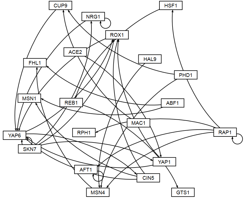
Section 2 above described how GRNsight uses the data in the adjacency matrix to automatically display a graph. This section describes how to interpret the results of the resulting gene regulatory network graph biologically, focusing on the demonstration files Demo #3: Unweighted GRN (21 genes, 31 edges) and Demo #4: Weighted GRN (21 genes, 31 edges, Schade et al. 2004 data). These two files describe gene regulatory networks from budding yeast, Saccharomyces cerevisiae, and correspond to supplementary data published in the paper, Dahlquist, K.D., Fitzpatrick, B.G., Camacho, E.T., Entzminger, S.D., and Wanner, N.C. (2015) Parameter Estimation for Gene Regulatory Networks from Microarray Data: Cold Shock Response in Saccharomyces cerevisiae. Bulletin of Mathematical Biology. 77: 1457-1492, published online 29 September 2015, DOI: 10.1007/s11538-015-0092-6, and when displayed by GRNsight, represent interactive versions of Figures 1 and 8 of that paper respectively.
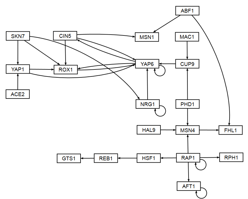
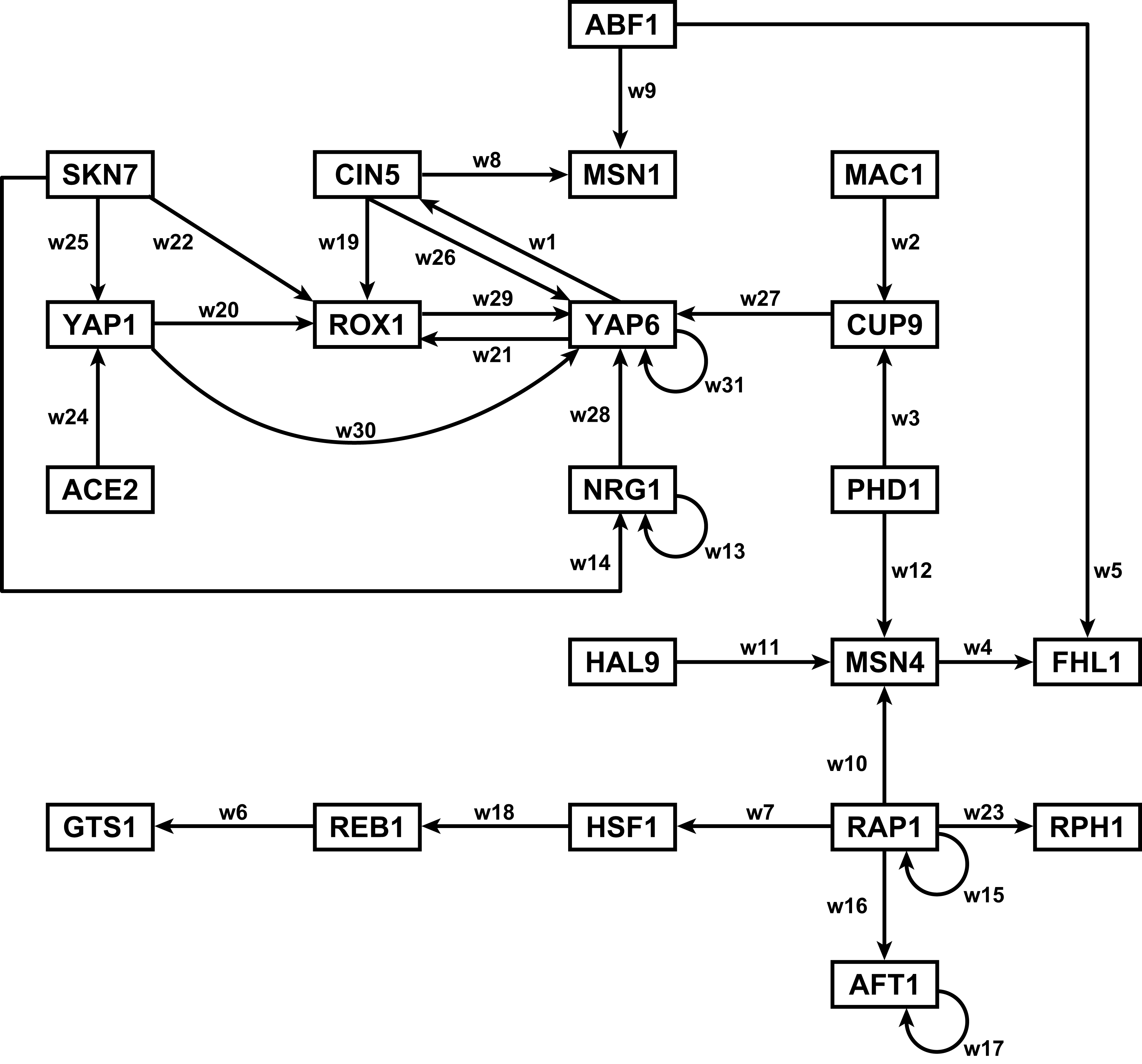
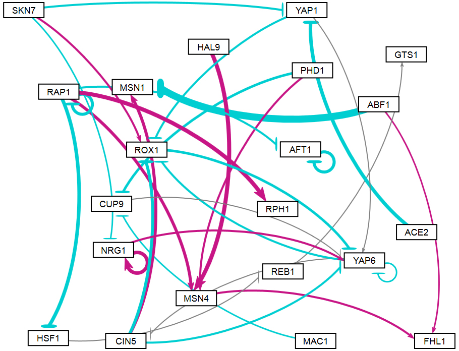
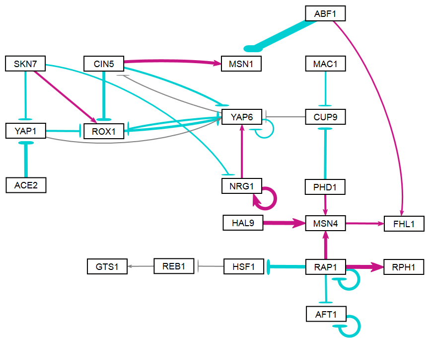
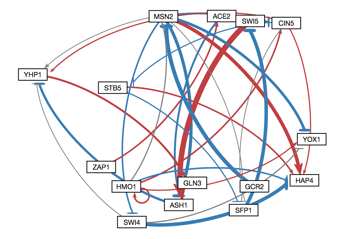
The figures shown below give a side-by-side view of the same adjacency matrices laid out by GRNsight and by hand. The top three figures are derived from Demo #3: Unweighted GRN (21 genes, 31 edges), and the bottom three panels are derived from Demo #4: Weighted GRN (21 genes, 31 edges, Schade et al. 2004 data). The left two panels show an example of the automatic layout performed by GRNsight. The right two panels show the same adjacency matrix laid out by hand in Adobe Illustrator, corresponding to Figure 1 (top right) and Figure 8 (bottom right) of the Dahlquist et al. (2015) paper. The middle two panels started with the automatic layout from GRNsight and then were manually manipulated from within GRNsight to lay them out similarly to the right-hand panels. The use of GRNsight represents a substantial time savings compared to creating the same figure entirely by hand.
 |
 |
 |
 |
 |
 |
- Viewing the unweighted network (top panel) allows one to make observations about the network structure. For example, YAP6 has the highest in-degree, being regulated by six other transcription factors. RAP1 has an out-degree of five, regulating four other transcription factors and itself. Four genes, AFT1, NRG1, RAP1, and YAP6, regulate themselves. Many of the transcription factors are involved in regulatory chains, with the longest including five nodes originating at SKN7. There are several other 4-node chains that originate at CIN5, MAC1, PHD1, SKN7, and YAP1. Finally, there are two feedforward motifs involving CIN5, ROX1, and YAP6 and SKN7, YAP1, and ROX1. More information about this network can be found in Dahlquist et al. (2015).
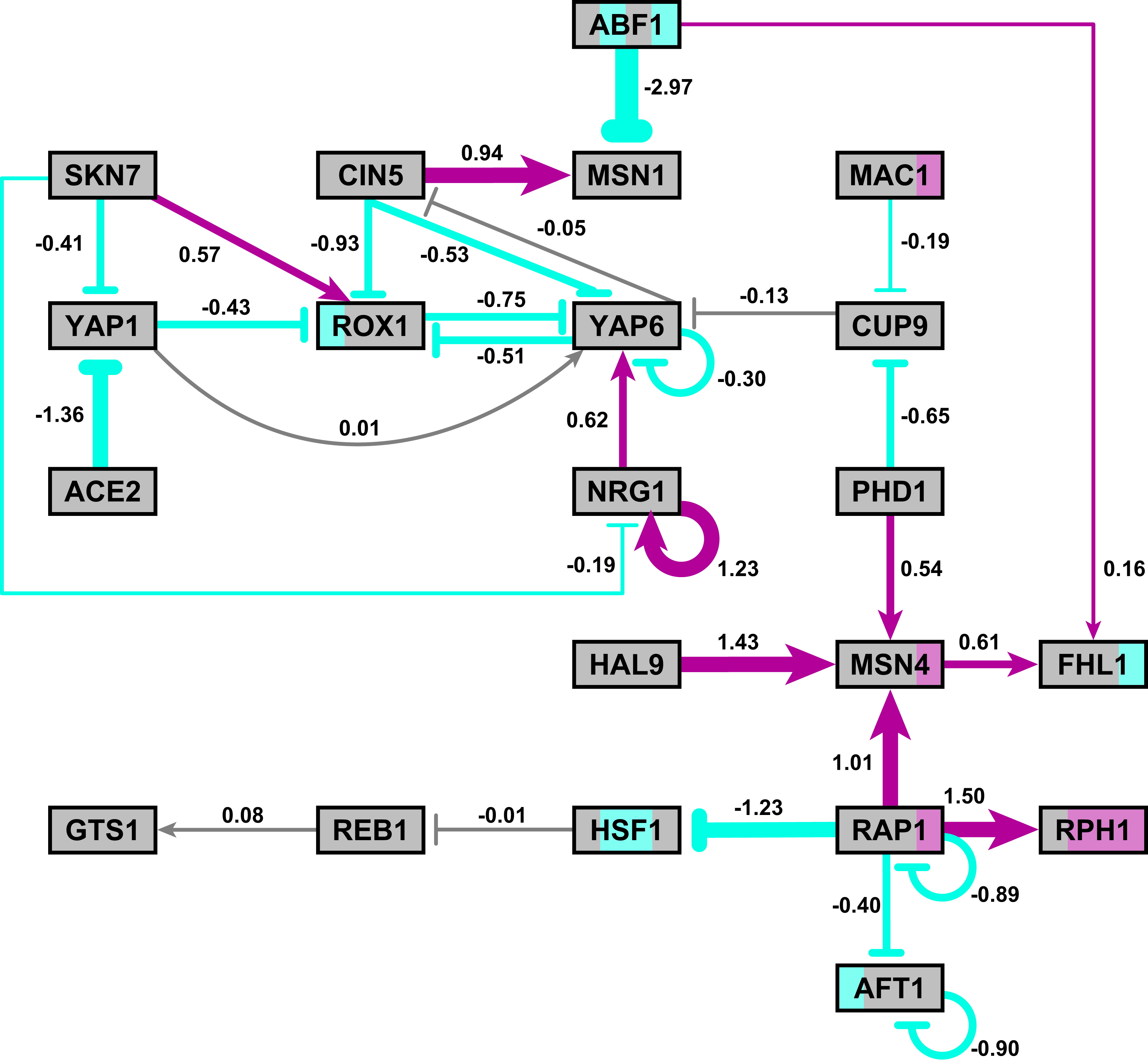
- The networks with colored edges shown in the bottom panel display the results of a mathematical model, called GRNmap, where the expression levels of the individual transcription factors were modeled using mass balance ordinary differential equations with a sigmoidal production function. Each equation in the model included a production rate, a degradation rate, weights that denote the magnitude and type of influence of the connected transcription factors (activation or repression), and a threshold of expression. The differential equation model was fit to published yeast cold shock microarray data from Schade et al. (2004) using a penalized nonlinear least squares approach. Model predictions fit the experimental data well, within the 95% confidence interval.
- In particular, GRNsight is displaying the results of the optimized weight parameters. Positive weights > 0 represent an activation relationship and are shown by regular (pointy) arrowheads. One example is that CIN5 activates the expression of MSN1. Negative weights < 0 represent a repression relationship and are shown by a blunt arrowhead (a line segment perpendicular to the edge direction). One example is that ABF1 represses the expression of MSN1.
- The thicknesses of the edges also vary based on the magnitude of the absolute value of the weight. Larger magnitudes have thicker edges and smaller magnitudes have thinner edges. The way that GRNsight determines the edge thickness is as follows. GRNsight divides all weight values by the absolute value of the maximum weight in the matrix to normalize all the values to between zero and 1. GRNsight then adjusts the thickness of the lines to vary continuously from the minimum thickness (for normalized weights near zero) to maximum thickness (normalized weights of 1). For example, in the bottom panel, the thickest edge corresponds to the repression of the expression of MSN1 by ABF1 because it has the highest magnitude weight parameter of -2.97.
- The color of the edge also imparts information about the regulatory relationship. Edges with positive normalized weight values from 0.05 to 1 are colored magenta (red in GRNsight >= v3.0.0). There are 10 magenta edges in this example. Edges with negative normalized weight values from -0.05 to -1 are colored cyan (blue in GRNsight >= v3.0.0). There are 16 cyan edges in this example. Edges with normalized weight values between -0.05 and 0.05 are colored gray to emphasize that their normalized magnitude is near zero and that they have a weak influence on the target gene (5 edges in this example).
- Because of this visualization of the weight parameters, one can make some interesting observations about the behavior of the network. The expression of several genes is controlled by a balance of activation and repression by different regulators. For example, the expression of MSN1 is strongly activated by CIN5, but even more strongly repressed by ABF1. Furthermore, some transcription factors themselves act both as activators of some targets and repressors of other targets. For example, RAP1 activates the expression of MSN4 and RPH1, but represses the expression of AFT1, HSF1, and itself. RAP1 is known to act as both an activator and a repressor. Thus, GRNsight enables one to interpret the weight parameters more easily than one could from the adjacency matrix alone. For more information about the interpretation of the model results, see Dahlquist et al. (2015).
- Note that the nodes in the bottom right panel of the figure are also colored, based on the time course of expression of that gene in the Schade et al. (2004) microarray data (stripes from left to right, 10, 30, and 120 minutes of cold shock, with magenta representing a significant increase in expression relative to the control at time 0, cyan representing a significant decrease in expression relative to the control, and gray representing no significant change in expression relative to the control). This feature is available in GRNsight >= v3.0.0, and described in the section below.
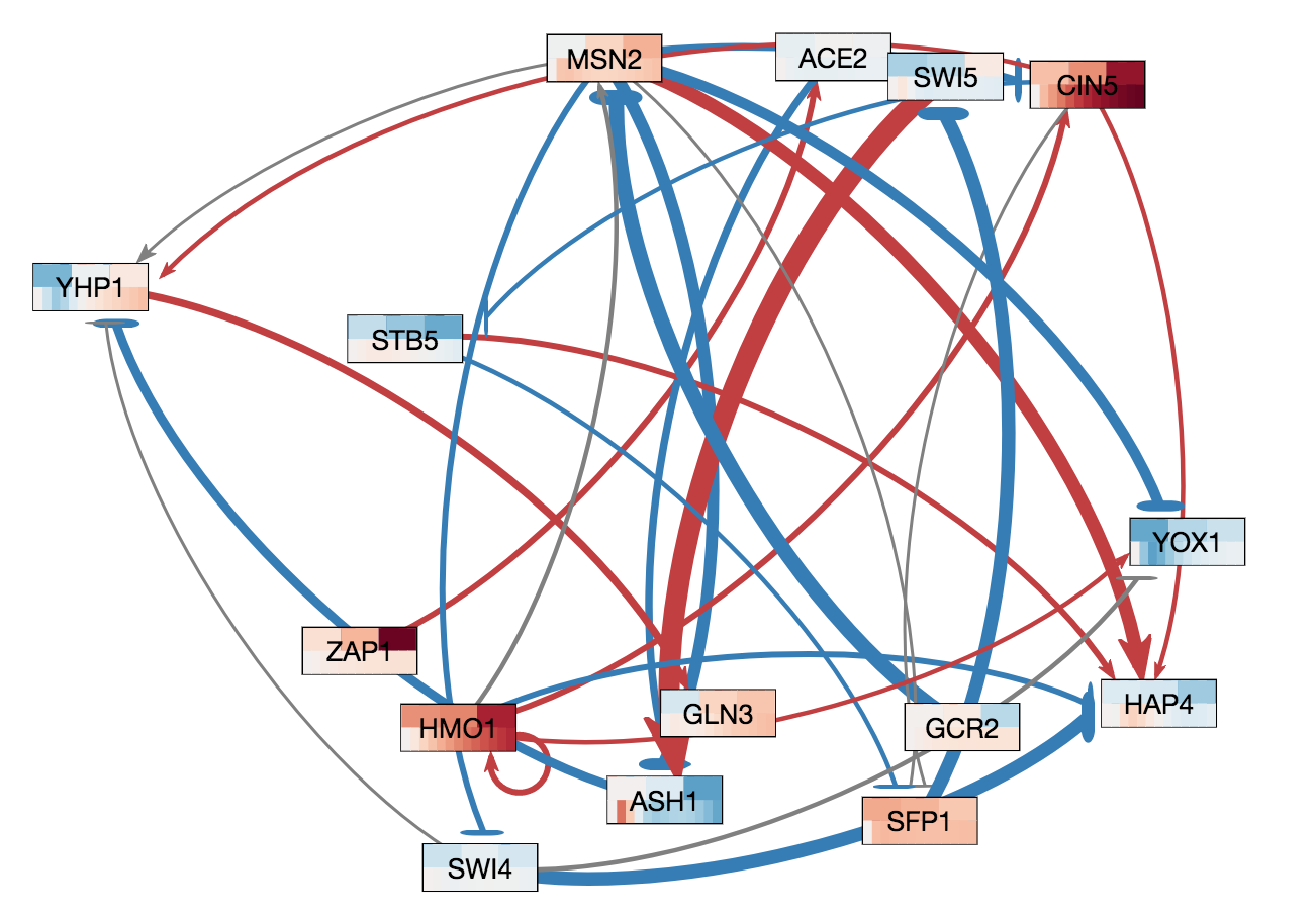
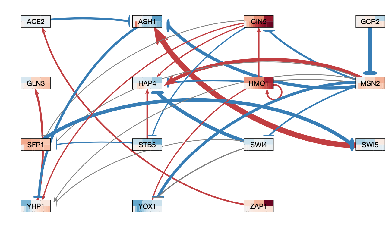
In GRNsight v3.0.0, two major features were added to GRNsight: node coloring visualization for time series expression data and a grid layout option. The following three figures were derived from Demo #2 Weighted GRN (15 genes, 28 edges, Dahlquist Lab unpublished data) using GRNsight v3.0.0. The figure on the left shows an example of the automated force graph layout generated by GRNsight with the new edge coloring scheme introduced in GRNsight v3.0.0. The figure in the middle shows an example of the automated force graph layout with the node coloring feature turned on. The figure on the right shows an example of the grid layout option with the node coloring feature turned on.
 |
 |
 |
- As shown in the figure on the left, the color scheme for edges was changed in GRNsight v3.0.0 to red and blue from magenta and cyan, respectively. The color scheme was changed to to provide more visual contrast over the original coloring scheme for color-blind users.
- Demo #2 Weighted GRN (15 genes, 28 edges, Dahlquist Lab unpublished data) contains expression sheets formatted for node coloring. Nodes in the graph are colored in the middle and left figure to visualize the level of expression of transcription factors over time. Two different datasets are selected for the top and bottom nodes to facilitate visual comparision between the expression values in the datasets. The top half of the nodes are colored using data from the sheet "wt_log2_expression" of Demo #2 and the bottom half of the nodes are colored using data from the sheet "wt_log2_optimized_expression" of Demo #2. The number of vertical node coloring slices in each half of the node correspond to the number of data points in the data set. The color of each vertical slice correspond to the color that the expression value at that time point maps to on the node coloring color scale, located in the sidebar menu of the user interface. By default, -3 maps to the darkest blue shade, while 3 maps to the darkest red shade.
- The figure on the right shows an example of the grid layout option. Grid layout was introduced in GRNsight v3.0.0 to provide an alternative graph layout option to the force graph layout. In grid layout mode, nodes are alphabetically organized in a grid pattern.
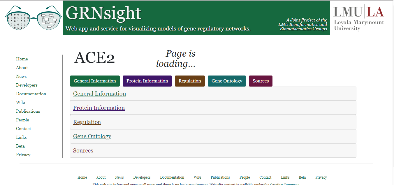
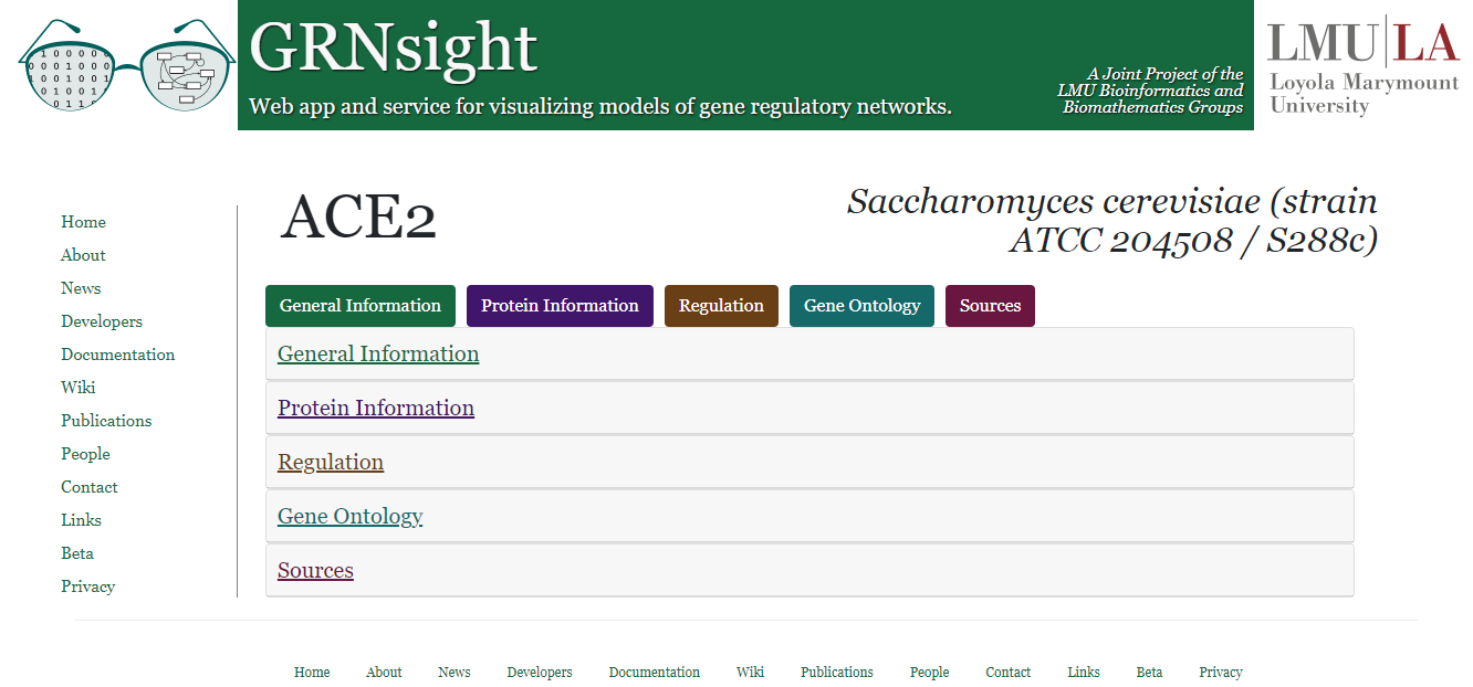
In GRNsight v3.1.0, the gene page feature was added. To access a gene page, right-click on the label of any given node when a graph is displayed. A "page is loading" message should appear while data is being retrieved from the source databases, as shown in the figure on the left.
 |
 |
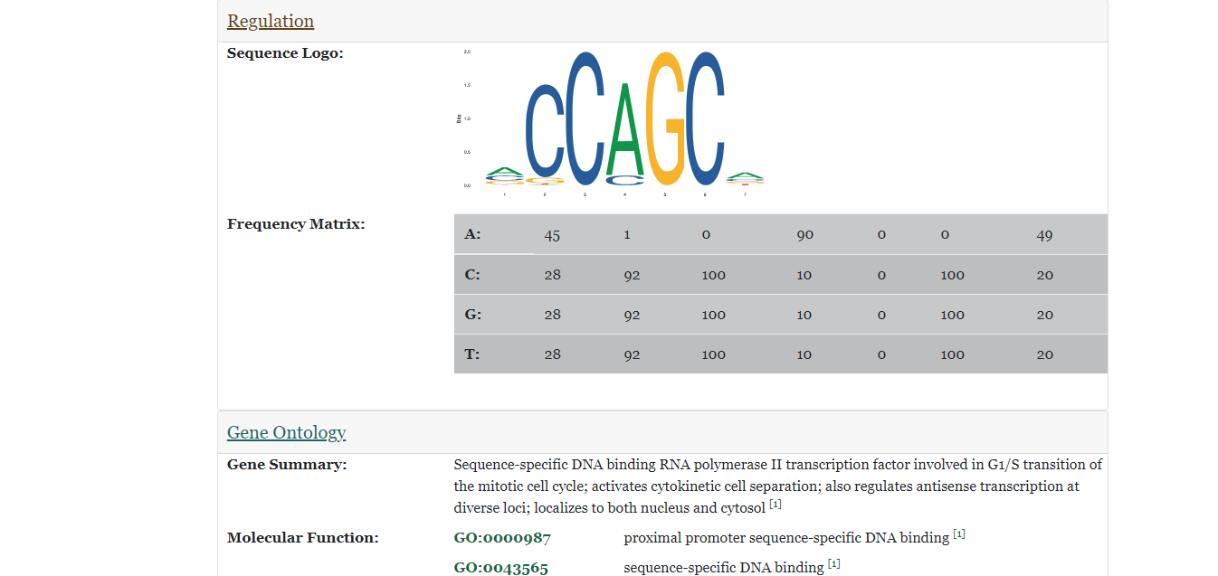 |
- The figure in the center shows the gene page when it is loaded. The gene name is displayed at top left. The species that the data is collected from is displayed at top right. Currently, this feature is limited to genes from Saccharomyces cerevisiae. The gene page pulls data from the UniProt, NCBI Gene, Ensembl, JASPAR, and the Saccharomyces Genome Database (SGD). Note, there is a known bug in GRNsight v7 where data from UniProt, Ensembl, JASPAR, SGD, and Gene Ontology are not displaying due to changes in the syntax in the API calls.
- The figure on the right displays that after clicking on a button corresponding to a certain section, the page is directed to that section and displays information about the specified information about the gene in the species. In this instance, a sequence logo and frequency matrix from the JASPAR database, and a list of Gene Ontology terms are displayed.
-
To export your data to SIF format, select the menu option Export > Export Data > To Unweighted SIF or File > Export Data > To Weighted SIF. A dialog box will open for you to Save your file. Clicking the Cancel button will return you to the GRNsight web page.
- When an unweighted GRN or PPI network is loaded, exporting to an unweighted SIF file will be the only option available.
- When a weighted GRN is displayed, you have the option to export to an unweighted or weighted SIF file. The difference between the unweighted and weighted SIF file is described below.
-
While there are several valid ways that a SIF file can be formatted for import into GRNsight (Section 1b-i.c), GRNsight follows a particular convention when exporting to SIF.
- GRNsight will export the network data as a tab-delimited text file (not space delimited) with a .sif file extension.
- The suggested filename for export will default to the same filename as was opened/imported with the file extension changed to .sif.
- If you are exporting a weighted network as an unweighted SIF file, the text "_unweighted" will be appended to the suggested filename before the file extension to denote this.
- For unweighted GRNs, the relationship type “pd” will be used. The relationship type of “pd” is used because it commonly means protein -> DNA (e.g. a regulatory transcription factor binding upstream of a target gene) in the systems biology community. For PPIs, the relationship type "pp" will be used. This default value cannot be changed from within GRNsight, but the exported SIF file could be edited in another program to do so.
- For weighted GRNs, if the user has selected the option of exporting the data as an unweighted network, the relationship type “pd” will be used.
- If the user has selected the option to export a weighted network as a weighted network, the numerical weight value for each edge is given as the relationship type.
- In each case, each line will consist of source node, relationship type, and target node, separated by tab characters. If a particular source node has multiple targets, they will be listed on separate lines. If a particular source node has no targets, it will still be listed on a separate line. The screenshots shown below are examples of how GRNsight exports Demo #3: Unweighted GRN (21 genes, 31 edges)" and Demo #4: Weighted GRN (21 genes, 31 edges, Schade et al. 2004 data)", respectively, to SIF files. (The screenshots display a tab-delimited text file as it would be displayed in Microsoft Excel.) Follow the links to download the sample SIF files.
- Note that these “weighted” SIF files are able to be imported in to Cytoscape (tested with v3.4.0), but the weight values will not be properly stored as edge attributes by Cytoscape because it does not use the SIF format in this way.
- One benefit from this export behavior is that GRNsight can be used to convert network data from an adjacency matrix (in the native GRNsight .xlsx format as described in Section 1b-i.a) to a list of binary interactions (as a SIF file).
- To export a GRN to GraphML format, select the menu option Export > Export Data > To Unweighted GraphML or File > Export Data > To Weighted GraphML. A dialog box will open for you to Save your file. Clicking the Cancel button will return you to the GRNsight web page. (Note that exporting PPI data to GraphML is not currently supported by GRNsight).
- When an unweighted GRN is loaded, exporting to an unweighted GraphML file will be the only option available.
- When a weighted GRN is loaded, you have the option to export to an unweighted or weighted GraphML file.
- The unweighted and weighted GraphML files will be formatted according to the description in Section 1b-i.d.
- To export your data to Excel format (.xlsx), select the top menu option Export > Export Data > To Excel. A modal window will appear allowing you to choose which data will be exported. The options are different for a GRN and a PPI. The goals of the GRN options are to create an Excel workbook that is compatible with the GRNmap MATLAB modeling software and also to be able to export a mirror of the user-uploaded data. Once you have made your selections, click the Export Workbook button. A dialog box will open for you to Save your workbook. Clicking the Cancel button will return you to the GRNsight web page.
- GRN:
- First, you can select the source of expression data. You have the option to export any of the expression datasets stored in the backend Expression database, your user-uploaded data, or none.
- From there you can select which particular worksheets you will export. Network sheets contain an adjacency matrix specifying the network as described in Section 1b-i.a. The network worksheet describes an adjancency matrix of 1's and 0's. The network_optimized_weights sheet contains the edge weight values. The network_weights sheet is a special worksheet required by the GRNmap modeling software that is described in the GRNmap documentation. The Expression Sheets contain the timecourse gene expression data from the Expression Data source selcted above. Additional sheets that can be exported are degradation_rates, optimization_parameters, production_rates, and threshold_b, which are all specific to the GRNmap software. mRNA degradation rates are derived from data published in Neymotin et al. (2014). mRNA production rates are supplied as double the degradation rates as initial guesses for the GRNmap modeling. The optimization_parameters and threshold_b are also used by GRNmap.
- The Excel workbooks will be formatted according to the description in Section 1b-i.a.
- To export your data as an image, select the menu option Export > Export Image > To [PNG, SVG, PDF]. A dialog box will appear, allowing you to save your file. Selecting Cancel will return you to the GRNsight web page.
- Note: it is known that when an GRNsight-exported SVG file is opened in Adobe Illustrator, it does not display properly. If you plan to use Adobe Illustrator, follow these steps:
- Download the graph as an SVG.
- Open the file in a web browser such as Chrome.
- Export it as a PDF from the browser.
- Open the PDF in Adobe Illustrator to view the vector graphic properly.
To print a graph, select the menu item File > Print. Mac users can utilize the native print to PDF function available from their operating system to print the graph to a PDF file. Windows users will need to have the full version of Adobe Acrobat (or other "print to PDF" utility) to print graphs to a PDF file. The Print menu item is disabled until a gene regulatory network graph is loaded. There is a known bug when GRNsight is used with Firefox browsers where the side of the graph gets cut off. This is an issue with Firefox that we cannot solve at this time. There are two workarounds. First, in Firefox, go to the menu item File > Page Setup and check the box Shrink to fit Page Width. Second, you can use the Chrome browser to print to PDF.
For additional documentation, please see the GRNsight Wiki.
To request support or features or report bugs, please submit an issue to GRNsight @ GitHub (requires free GitHub account).